17.3.1999
Mikko Kokkonen, 33015p

Solutions to exercises 3

Exercise 2.2

Maple-solution in HTML

Exercise 2.8

Maple-solution in HTML

Exercise 2.14c

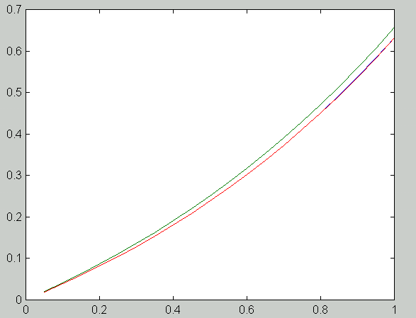
The image below shows the solutions of the boundary value problem. The blue curve is the true solution, the green curve is the numerical solution obtained with scheme 1 and the red curve is the solution obtained with scheme 2. Here n = 19.

Estimation of the rate of convergence (using the technique of Project 1.1 that has been implemented in a Matlab-script):

       n	 h	 E_h1	   E_h2	      R_1	R_2
    4.0000    0.2000	0.0946    0.0054
    9.0000    0.1000    0.0486    0.0014    0.9592    1.9987
   19.0000    0.0500    0.0247    0.0003    0.9800    1.9997
   49.0000    0.0200    0.0099    0.0001    0.9910    1.9999
   99.0000    0.0100    0.0050    0.0000    0.9961    2.0000

The scheme 2 converges faster because the two-sided finite difference approximation of the first derivative is more accurate than the one-sided (backward) approximation used in the scheme 1.

Exercise 2.17

Here f(x) = 100 exp(-10x). Hence f'(x) = -1000 exp(-10x), f''(x) = 10000 exp(-10x) and || f'' ||_infty = 10000. The error estimate given by Theorem 2.2 is in this case || u - v ||_infty <= 10000 h^2 / 96. Comparison to actual value of the max difference between the analytic and numeric solution is shown in the table below:

               True      Error
       h      error    estimate
    0.1000    0.0527    1.0417
    0.0500    0.0137    0.2604
    0.0250    0.0035    0.0651
    0.0125    0.0009    0.0163
    0.0062    0.0002    0.0041

The lesson of this exercise is that if the f'' has a large maximum value compared to the average value of the function, then Theorem 2.2 can largely overestimate the actual error.

Project 2.2

Plots of numerical (circles) and analytic (curve) solutions to the boundary-value problem (with n=100):

alpha = 1:
alpha = 5:
alpha = 100:

Numerical estimation of the rate of convergence (using the technique of Project 1.1):

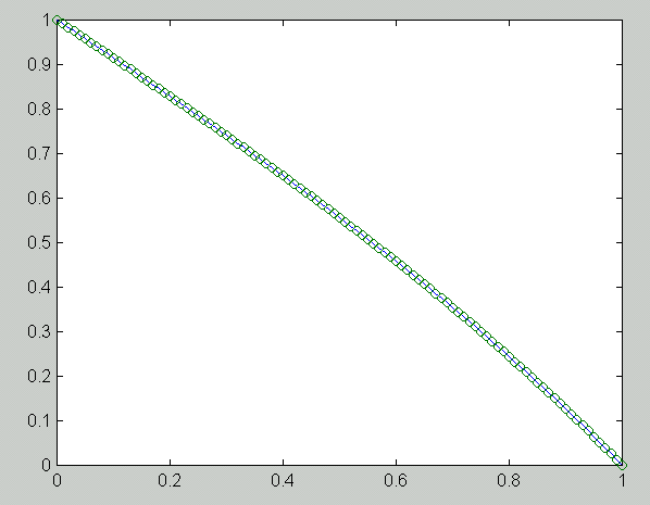
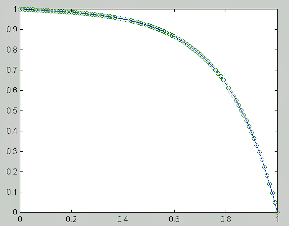
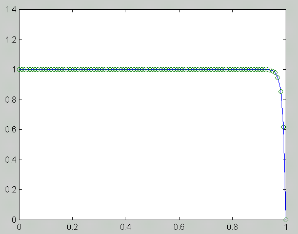
   n        h       e_1       e_5      e_100       R_1       R_5     R_100
    4    0.2000    0.0002    0.0140    0.0025
    9    0.1000    0.0000    0.0037    0.0098    1.9946    1.9100   -1.9721
   19    0.0500    0.0000    0.0010    0.0304    1.9986    1.9758   -1.6368
   49    0.0200    0.0000    0.0002    0.0362    1.9997    1.9948   -0.1935
   99    0.0100    0.0000    0.0000    0.0141    1.9993    1.9990    1.3632
  199    0.0050    0.0000    0.0000    0.0037    2.0000    1.9998    1.9105
  399    0.0025    0.0000    0.0000    0.0010    1.9999    1.9999    1.9759