8.4.1999
Mikko Kokkonen, 33015p

Solutions to exercises 5

Exercise 1.

The problem with the maple-worksheet seems to be in the plotting part, because the values U[i] (which are equal to the numerical solution evaluated at x[i]) are nearly equal (within high precision) to the true solution.

Exercise 2.

The results from the debugged and completed matlab-solution for the FEM problem and from the finite difference solution are shown below:

 x           0.1667    0.3333    0.5000    0.6667    0.8333
true sol.    0.1641    0.3101    0.4122    0.4328    0.3196
FEM sol.     0.1641    0.3101    0.4122    0.4328    0.3196
fd sol.      0.1613    0.3054    0.4063    0.4271    0.3156

At the grid points the FEM produces much more accurate results in comparison to the finite difference solution when h is large, because the the stiffness matrix is exact and the load vector in computed to a high precision with the adaptive numerical integration method of matlab (quad8).

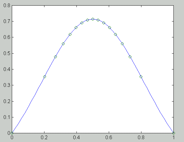
The following figure has been produced with the matlab-solution for the equation of the exercise 1. The solid curve is the exact solution and the circles represent the FEM solution at the grid points.

Exercise 3.

a. The code for solving the Sturm-Liouville equation is available at the moment for the following two cases (the rest will be completed shortly):

homogenous Dirichlet boundary conditions,
mixed boundary conditions with Dirichlet type condition at x=0 and Neumann type condition at x=1.

They use the trapetzoidal rule (2 function evaluations for each integral) for computing the elements of the stiffness matrix and the load vector.

b. Convergence rate of FEM with trapetzoidal integration rule has been estimated using a matlab-script and data from [T-W] exercise 2.14. Results below indicate that the rate of convergence is O(h ²).

      n          h       error     rate 
    5.0000    0.2000    0.0054
   10.0000    0.1000    0.0014    1.9987
   20.0000    0.0500    0.0003    1.9997
   50.0000    0.0200    0.0001    1.9999
  100.0000    0.0100    0.0000    2.0000

Exercise 4.

The solution for the Exercise 9.2.5 with the PDEtool of matlab is shown in the figure below (the solution can be reproduced with this matlab-script):

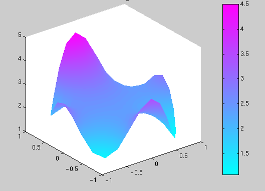
This can be compared with the solutions obtained with Fourier series or direct integration of the Poisson kernel.

The table below shows how the error (with respect to the exact solution) at grid points behaves as the mesh is refined. Each refinement reduces the error by a factor approximately equal to three.

               Max error
Original mesh  0.0106
1st refinement 0.0035
2nd refinement 0.0011
3rd refinement 3.3824e-04