Lämpöyhtälö muuttujat erotellen
Numsym 15.2.2005
Alustukset
| > |
with(plots): setoptions3d(orientation=[-120,50],axes=box):
|
Warning, the name changecoords has been redefined
Esim
KRE s. 603
Exa 1
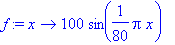
| > |
f:=x->100*sin(Pi*x/80); plot(f,0..80);
|
![[Maple Plot]](images/lampoyhtalo2.gif)
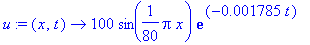
| > |
u:=(x,t)->100*sin(Pi*x/80)*exp(-0.001785*t);
|
| > |
plot3d(u(x,t),x=0..80,t=0..400,axes=box);
|
![[Maple Plot]](images/lampoyhtalo4.gif)
"Aikasiivuparvi" :
| > |
[seq(u(x,t),t=[seq(i*0.1,i=0..5)])];
|
![[100.*sin(1/80*Pi*x), 99.98215159*sin(1/80*Pi*x), 99.96430637*sin(1/80*Pi*x), 99.94646434*sin(1/80*Pi*x), 99.92862548*sin(1/80*Pi*x), 99.91078982*sin(1/80*Pi*x)]](images/lampoyhtalo5.gif)
Tällainen lausekkeiden lista voidaan antaa suoraan
plot:
lle, kuten tiedämme: Otetaan samantien enemmän aikaviipaleita.
| > |
plot([seq(u(x,t),t=[seq(i*30,i=0..10)])],x=0..80);
|
![[Maple Plot]](images/lampoyhtalo6.gif)
| > |
animate(u(x,t),x=0..80,t=0..400,frames=30);
|
![[Maple Plot]](images/lampoyhtalo7.gif)
Exa 2. Muuten sama, mutta nyt
| > |
restart:with(plots): setoptions3d(orientation=[-120,50],axes=box):
|
Warning, the name changecoords has been redefined
| > |
f:=x->100*sin(3*Pi*x/80); plot(f,0..80);
|

![[Maple Plot]](images/lampoyhtalo9.gif)
![lambda[3] := 3*c*Pi/L](images/lampoyhtalo10.gif)
| > |
c:=sqrt(1.158):L:=80: lambda[3];
|
| > |
u:=(x,t)->100*sin(3*Pi*x/L)*exp(-lambda[3]^2*t);
|
![u := proc (x, t) options operator, arrow; 100*sin(3*Pi*x/L)*exp(-lambda[3]^2*t) end proc](images/lampoyhtalo12.gif)
| > |
plot3d(u(x,t),x=0..80,t=0..200,axes=box);
|
![[Maple Plot]](images/lampoyhtalo13.gif)
"Aikasiivuparvi" :
| > |
#[seq(u(x,t),t=[seq(i*0.1,i=0..5)])];
|
Tällainen lausekkeiden lista voidaan antaa suoraan
plot:
lle, kuten tiedämme: Otetaan samantien enemmän aikaviipaleita.
| > |
plot([seq(u(x,t),t=[seq(i*20,i=0..10)])],x=0..80);
|
![[Maple Plot]](images/lampoyhtalo14.gif)
| > |
animate(u(x,t),x=0..80,t=0..200,frames=30);
|
![[Maple Plot]](images/lampoyhtalo15.gif)
Muuttujien erottelu
| > |
restart:
with(LinearAlgebra): with(plots):
|
Warning, the name changecoords has been redefined
| > |
setoptions3d(orientation=[-120,50],axes=box):
|
| > |
#read("c:\\usr\\heikki\\numsym05\\maple\\ns05.mpl");
|
| > |
# read("/p/edu/mat-1.192/ns05.mpl");
|
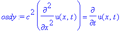
| > |
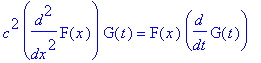
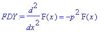
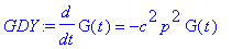
osdy:=c^2*diff(u(x,t),x$2)=diff(u(x,t),t);eval(subs(u(x,t)=F(x)*G(t), osdy));
|
| > |
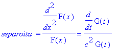
separoitu:=simplify(%/(c^2*F(x)*G(t)));
|
| > |
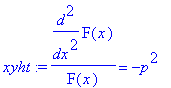
xyht:=lhs(separoitu)=-p^2;
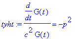
tyht:=rhs(separoitu)=-p^2;
|
| > |
FDY:=lhs(xyht)*F(x)=rhs(xyht)*F(x);
|
| > |
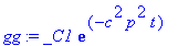
GDY:=c^2*lhs(tyht)*G(t)=c^2*rhs(tyht)*G(t);
|
| > |
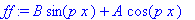
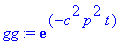
ff:=rhs(dsolve(FDY,F(x)));
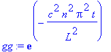
dsolve(GDY,G(t)): gg:=rhs(%);
|

| > |
ff:=subs(_C2=A,_C1=B,ff); gg:=subs(_C1=1,gg);
|
RE1 & RE2 ==>
| > |
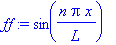
ff:=subs(A=0,B=1,p=n*Pi/L,ff);
|
| > |
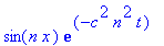
u:=sum(B[n]*ff*gg,n=1..infinity);
|
![u := sum(B[n]*sin(n*Pi/L*x)*exp(-c^2*n^2*Pi^2/L^2*t),n = 1 .. infinity)](images/lampoyhtalo30.gif)
Sinisarjaksi:
Alkuehto saadaan toteutumaan valitsemalla B[n]:t AE-funktion f (2L-jaksoisen) sinisarjan kertoimiksi.
Määritellään sinisarjan kertoimet ja annetaan alkuarvofunktion f sekä jakson puolikkaan L olla
vapaita, myöhemmin annettavia symboleja (vrt. fourier.mws-työarkki).
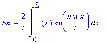
| > |
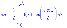
f:='f':L:='L':n:='n':Bn:=(2/L)*Int(f(x)*sin(n*Pi*x/L),x=0..L);
|
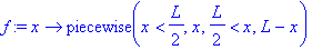
Otetaan esimerkiksi KRE s. 648, Exa 3
| > |
f:=x->piecewise(x<L/2,x,x>L/2,L-x);L:=Pi;
|

![[Maple Plot]](images/lampoyhtalo34.gif)
 :n pituinen sauva sopiii matemaatikoille.
| > |
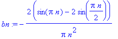
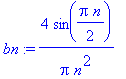
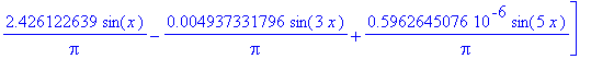
bn:=simplify(value(Bn));
|
| > |
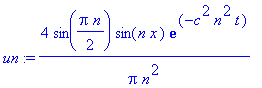
summaf:=(x,t,N)->add(un,n=1..N);
|


| > |
plot3d(summaf(x,t,5),x=0..Pi,t=0..2,axes=box);
|
![[Maple Plot]](images/lampoyhtalo43.gif)
Summafunktion "aikasiivuparvi" :
| > |
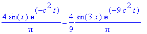
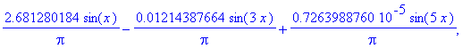
[seq(summaf(x,t,5),t=[seq(i*0.1,i=0..5)])];
|


Tällainen lausekkeiden lista voidaan antaa suoraan
plot:
lle, kuten tiedämme: Otetaan samantien enemmän aikaviipaleita.
| > |
plot([seq(summaf(x,t,40),t=[seq(i*0.1,i=0..10)])],x=0..Pi);
|
![[Maple Plot]](images/lampoyhtalo49.gif)
| > |
animate(summaf(x,t,40),x=0..Pi,t=0..10,frames=30);
|
![[Maple Plot]](images/lampoyhtalo50.gif)
Eristetyt päät, adiabaattiset reunaehdot
| > |
restart:
with(plots):setoptions3d(orientation=[-120,50],axes=box):
|
Warning, the name changecoords has been redefined
| > |
#read("c:\\usr\\heikki\\numsym05\\maple\\ns05.mpl");
|
| > |
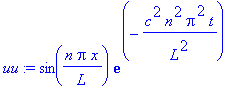
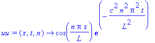
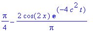
uu:=(x,t,n)->cos(n*Pi*x/L)*exp(-(c*n*Pi/L)^2*t);
|
| > |
usum:=(x,t,N)->add(a(n)*uu(x,t,n),n=0..N);
|

| > |
f:='f':L:='L':n:='n':an:=(2/L)*Int(f(x)*cos(n*Pi*x/L),x=0..L);
|
Esimerkiksi KRE s. 64x, Exa 4
| > |
f:=x->piecewise(x<L/2,x,x>L/2,L-x);L:=Pi;
|


![[Maple Plot]](images/lampoyhtalo57.gif)
| > |
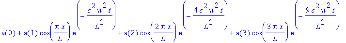
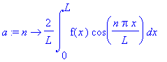
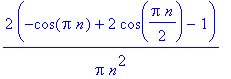
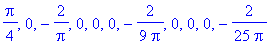
a:=n->2/L*int(f(x)*cos(n*Pi*x/L),x=0..L);
|
| > |
a(0):=1/L*int(f(x),x=0..L);
|


| > |
plot3d(usum(x,t,20),x=0..Pi,t=0..2,axes=box);
|
![[Maple Plot]](images/lampoyhtalo65.gif)
Summafunktion "aikasiivuparvi" :
| > |
#[seq(usum(x,t,20),t=[seq(i*0.1,i=0..5)])];
|
Tällainen lausekkeiden lista voidaan antaa suoraan
plot:
lle, kuten tiedämme: Otetaan samantien enemmän aikaviipaleita.
| > |
plot([seq(usum(x,t,10),t=[seq(i*0.1,i=0..10)])],x=0..Pi);
|
![[Maple Plot]](images/lampoyhtalo66.gif)
| > |
animate(usum(x,t,20),x=0..Pi,t=0..2,frames=30);
|
![[Maple Plot]](images/lampoyhtalo67.gif)