Date: 14.5.1999
Janne Viljas

Final project: QUADRATIC ELEMENTS for Matlab's PDE toolbox

Documentation

Documentation is available in .tex-, .dvi- or .ps-format. When I've had the time to learn, or if somebody teaches me to use the latex2html converter, I might make html yet another choise... A related Maple sesssion also exists both in html and as the original worksheet.

M-files

The Matlab .m-files can be found in this directory.

Instructions

There are some instructions in the above documentation, but the comments in the .m-files themselves should be sufficient.

The following is an extract from the LaTeX document:

If it wasn't clear from the beginning, I should say now that the purpose of this project was to expand the capabilities of Matlab's PDE toolbox to the realm of quadratic elements. The toolbox itself is still needed in order to take advantage from these additions. The expansion consists of essentially four functions. Their descriptions are given below:

qmesh, This function is written by Heikki Laitinen. It is so good as-is that there was no point in rewriting it. It transforms the mesh data structures p, e and t created by pdetool to a form suitable for quadratic elements.
qassema, forms the global K, M and F without worrying about Dirichlet boundary conditions.
qassemb, forms the global Q and G plus a vector R, which contains the values of the solution at the Dirichlet boundary nodes.
qassempde, This is the main function, which uses the two previous functions and then eliminates the equations corresponding to Dirichlet boundary conditions from the linear system. It gives out the final coefficient matrix and the rhs vector --- a system which can be solved to get the final solution of the problem.

So, to use the quadratic elements one should always first define the equations, boundary conditions and the geometry with the pdetool GUI, for example, and then run qmesh to transform the mesh. Then run qassempde and produce the solution. The function I have made to plot the solution is quite archaic, but it works; it is called qplotsol.

I also completed the linear element functions lassema, lassemb and lassempde, much of whose structure was already given on the course WWW-page. I shall include them with the ``quadratic functions'', but will not comment on them further. The quadratic functions were constructed to follow same principles as they do.

Examples

Example 1: Stuff... in a... pipe?

This involves the geometry from Celia-Gray that appeared before. It is a solution to the Poisson's equation

u_xx + u_yy + 2u = 10

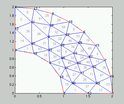
in the pipe-like region, whose element triangulation (plotted with pdeplotn) is shown in the first image. On the boundaries from 1 to 2, 3, to 4 and 2 to 3 we have the Dirichlet condition

u = x.*y.^2

and on the boundary from 1 to 4 the Neumann condition

u_n + 2yu = x.

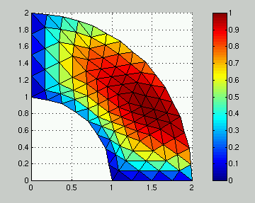
Note that this problem describes absolutely nothing at all. The second image still shows its solution using qassempde, which is plotted with the qplotsol function. The geometry is described in this .m-file.

Example 2: Candypotential modeled with Poisson's equation

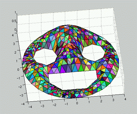
This is a solution of the Poisson's equation with zero boundary conditions and uniform unit source. Look at those cute random colors! The geometry is described in the .m-file given here.

Example 3: [not here yet]

I've been thinking of making this a useful one.