quadratic.html

Local K,M,F,Q and G - Quadratic shape functions

> restart:with(linalg):with(plots):

Warning, new definition for norm

Warning, new definition for trace

O.K. This is old stuff... the linear shape functions, or the triangle coordinates:

> cartesian:=vector([1,x,y]):natural:=vector([L1,L2,L3]):transform:=array([[1,1,1],[x1,x2,x3],[y1,y2,y3]]):

> op(cartesian)=evalm(transform&*natural):

> itr:=inverse(transform):

> LL:=evalm(itr&*cartesian):

> L1:=subs(denom(LL[1])=2*A,LL[1]):
L2:=subs(denom(LL[2])=2*A,LL[2]):
L3:=subs(denom(LL[3])=2*A,LL[3]):

Now the quadratic functions in terms of the linear shape functions

> psi[1]:=2*L1*(L1-1/2):psi[2]:=2*L2*(L2-1/2):
psi[3]:=2*L3*(L3-1/2):psi[4]:=4*L2*L3:
psi[5]:=4*L1*L3:psi[6]:=4*L1*L2:

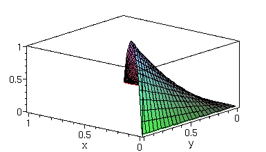
One of them looks like this:

> psii:=subs(A=-(-x2*y3+x3*y2+x1*y3-x1*y2-y1*x3+y1*x2)/2,psi[4]):plot3d(subs(x1=0,y1=0,x2=1,y2=0,x3=0,y3=1,psii),x=0..1,y=0..1-x,axes=boxed,orientation=[130,60]);

The elements of the 6x6 matrices K,M and the 6x1 vector F require area integrations over the element triangle. We approximate the integrals with the midpoint quadrature (accuracy order 3, optimal for quadratic elements)

where A is the area of the triangle and the middle points are numbered from 4 to 6 in the usual way. Note that henceforth the functions h are needed in these points only and that makes life a lot easier.

On the other hand, evaluation of the matrix Q and vector G involve 1D integrals over element sides. For them we use the Simpson quadrature (accuracy order 4, superoptimal by one)

where L is the length of the triangle edge and Pa,Pb plus Pc are the edge endopoints and the midpoint, respectively.

We will consider the stiffness matrix K first.

Stiffness matrix K

For this we need the gradients of the local shape functions...

> for i to 6 do
g[i]:=simplify([diff(psi[i],x),diff(psi[i],y)]): od:

Middle points of the triangular element sides

> x4:=(x2+x3)/2:x5:=(x1+x3)/2:x6:=(x1+x2)/2:
y4:=(y2+y3)/2:y5:=(y1+y3)/2:y6:=(y1+y2)/2:

and the gradients evaluated at those points P, denoted awkwardly by gat<P>[i]:

> for i to 6 do
gat4[i]:=simplify(subs(x=x4,y=y4,A=-(-x2*y3+x3*y2+x1*y3-x1*y2-y1*x3+y1*x2)/2,g[i])): od:
for i to 6 do
gat5[i]:=simplify(subs(x=x5,y=y5,A=-(-x2*y3+x3*y2+x1*y3-x1*y2-y1*x3+y1*x2)/2,g[i])): od:
for i to 6 do
gat6[i]:=simplify(subs(x=x6,y=y6,A=-(-x2*y3+x3*y2+x1*y3-x1*y2-y1*x3+y1*x2)/2,g[i])): od:

These are all we need for the quadrature when evaluating the local stiffness matrix. Let us still simplify them by substituting A for the previously obtained area expression, and we are done:

> for i to 6 do
gat4[i]:=subs(denom(gat4[i][1])=2*A,gat4[i]); od;
for i to 6 do
gat5[i]:=subs(denom(gat5[i][1])=2*A,gat5[i]); od;
for i to 6 do
gat6[i]:=subs(denom(gat6[i][1])=2*A,gat6[i]); od;

And now the components are (c is a 2x2 matrix or a scalar), if the notation makes any sense at all, something like

(The g_i's are the gradients of the i'th shape functions.)

Mass matrix M

So much for the stiffness matrix. Now let us see what the local mass matrix looks like in the ideal case, i.e. when a=1:

> L1:='L1':L2:='L2':L3:='L3':

> 2*'A'*int(int(4*Li*(Li-1/2)*Li*(Li-1/2),Lj=0..1-Li),Li=0..1);

> 2*'A'*int(int(4*Li*(Li-1/2)*Lj*(Lj-1/2),Lj=0..1-Li),Li=0..1);

> 2*'A'*int(int(16*Li*Lj*Li*Lj,Lj=0..1-Li),Li=0..1);

> 2*'A'*int(int(16*Li*(1-Li-Lj)*Li*Lj,Lj=0..1-Li),Li=0..1);

> 2*'A'*int(int(8*Li*Lj*Li*(Li-1/2),Lj=0..1-Li),Li=0..1);

> M:='A'/15*matrix(6,6,[1/2,-1/12,-1/12,0,0,0,-1/12,1/2,-1/12,0,0,0,-1/12,-1/12,1/2,0,0,0,0,0,0,8/3,4/3,4/3,0,0,0,4/3,8/3,4/3,0,0,0,4/3,4/3,8/3]);

And that's it. However, we won't be needing this, as we will be using the midpoint quadrature for the case of general a. In that case M will clearly be diagonal:

for i,j=4,5,6 and zero otherwise.