15.2.1999
Mikko Kokkonen, 33015p
a. Proof by induction on n. Substituting 0 for n gives the initial values, so the result is true for n=0. Assuming result is true for some n, we have:
u(j,n+1) = (1 + c/rho) u(j,n) - c/rho u(j+1,n)
         = (1 + c/rho) (1 + 2c/rho)^n (-1)^j -
	        c/rho (1 + 2c/rho)^n (-1)^(j+1)
	 = (1 + 2c/rho) (1 + 2c/rho)^n (-1)^j
	 = (1 + 2c/rho)^(n + 1) (-1)^j.
b. As previously, the equation with n=0 gives the inital data. The induction step:
u(j,n+1) = (1 - c/rho) u(j,n) + c/rho u(j-1,n)
         = (1 - c/rho) (1 - 2c/rho)^n (-1)^j +
	        c/rho (1 - 2c/rho)^n (-1)^(j-1)
	 = (1 - 2c/rho) (1 -2c/rho)^n (-1)^j
	 = (1 - 2c/rho)^(n+1) (-1)^j.
CFL condition:
Delta x / Delta t >= c_max = max |c(f(x))|, where c(u) = u + 1 and
f(x) = x / (1 + x^2).
Derivating c(f(x)) with respect to x gives
D c(f(x)) = (1 + x^2 - x 2x) / (1 + x^2)^2The zeros of the derivative are +/- 1, the maximum value is reached at x=1 and c_max = 3/2. The CFL condition is in this case:
Delta x / Delta t >= 3/2
a. Upwind scheme with F(u) = u(beta - u) is
u(j,n+1) = u(j,n) - 1/rho [F(u(j,n)) - F(u(j-1,n))]
         = u(j,n) - [u(j,n)(beta - u(j,n)) - u(j-1,n)(beta - u(j-1,n))]/rho
	 = u(j,n) - [beta(u(j,n) - u(j-1,n)) - (u(j,n)^2 - u(j,n-1)^2)]/rho
b. To guarantee that the speed c is >= 0, we must have
c(f(x)) = beta - 2 f(x) >= 0which means that the initial value must satisfy the relation f(x) <= beta/2.
c. We need to compute c_max for the CFL:
c_max = max |c(f(x))| = max | beta - 2 f(x)| with 0 <= f(x) <= beta/2
      = beta
The CFL condition is thus
Delta x / Delta t >= beta
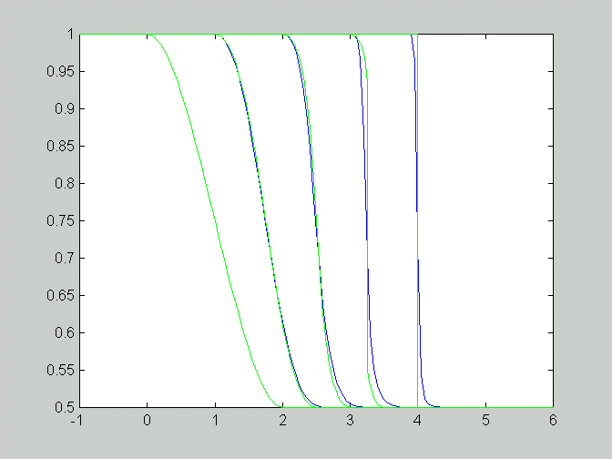
a. The figure below compares results from the method of characteristics
(green curves) and the numerical scheme (blue curves, step size: Delta x =
Delta t = 0.05). Differences between results increase with increasing time
because the errors caused by the finite difference approximation accumulate.

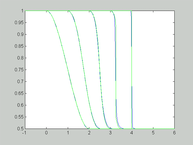
b. Decreasing the step size gives better results as the figure below
shows.
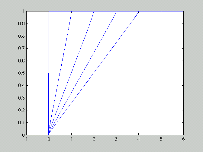
More comparisons between the method of characteristics and the numerical method with different initial values (Delta x = Delta t = 0.02, t = 1,2,3,4):
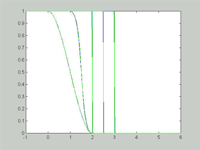
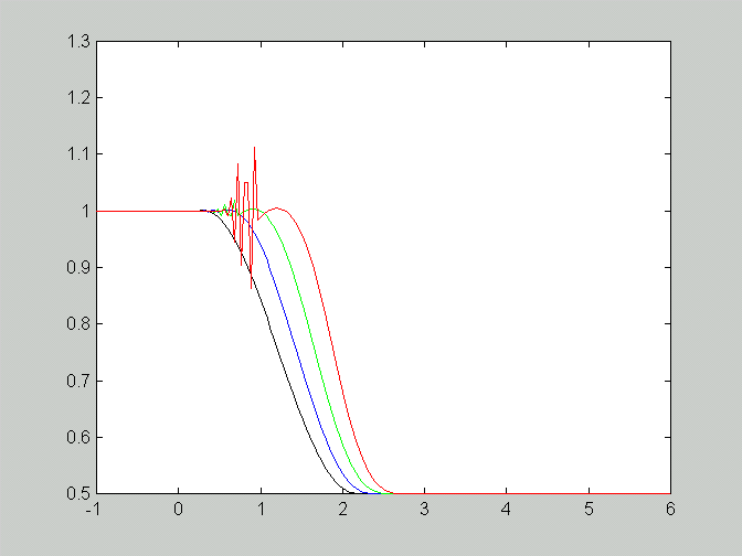
This figure shows what happens when the CFL condition is not satisfied:
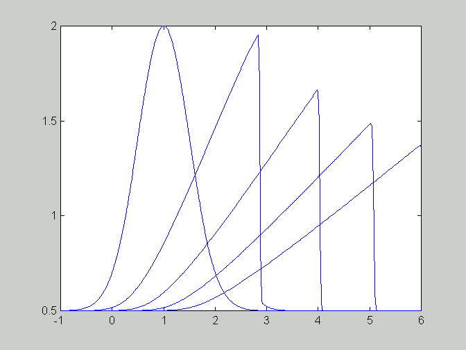
a. We need to compute c_max for the initial value f5(x) = 3/2 exp(-2(x-1)^2) + 1/2. The maximum value is c_max = f5(1) = 2 and the time step can be now derived from the CFL condition:
Delta t <= Delta x / 2The figure shows numerical results with Delta x = 0.02, Delta t = 0.01 and t=1,2,3,4.
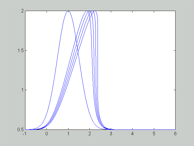
b. The shock appears first at t* = 1/max[-f5'(x)]. To find t* we need to compute first and second derivative of f5(x). The first derivative:
f5'(x) = -6 (x-1) exp(-2(x-1)^2)The second derivative:
f5''(x) = [24(x-1)^2 - 6] exp(-2(x-1)^2)The zeros of the 2nd derivative are 1/2 and 3/2. The maximum value is reached at x=3/2 and t* = - 1/f5'(3/2) = exp(1/2)/3 approx 0.55. The figure shows the solution near the appearance of shock (Delta x = 0.0025, Delta t = 0.00125, t=0.4375, 0.5, 0.5625, 0.625):
c. Behaviour of the shock after the formation is shown in this figure.
(Delta x = 0.01, Delta t = 0.005, t=0.5, 1, 1.5, 2, 2.5, 3, 3.5)
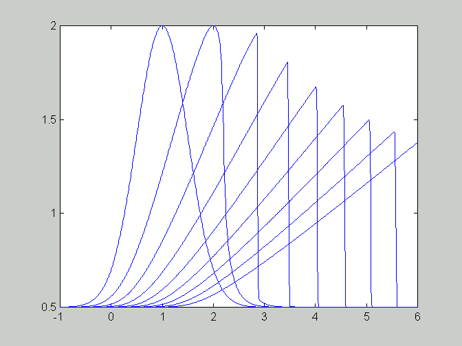
d. The speed of the shock can be calculated from the Rankine-Hugoniot condition:
s(t) = (F(u_l) - F(u_r)) / (u_l - u_r)where u_l is the value of the solution on the left of the discontinuity and u_r is value on the right hand side. By picking the values of u_l and u_r from the previous figure we can estimate the speed of shock:
t   | u_l  u_r  s
-------------------
1.0 | 1.96  0  0.98
2.0 | 1.68  0  0.84
3.0 | 1.50  0  0.75
4.0 | 1.38  0  0.69
a. Here initial values are defined as
f6(x) = 2(x-1) exp(-4(x-1)^2) + 1/2By looking at the plot of f6(x) we might expect something more than a single shock and rarefaction to develop.
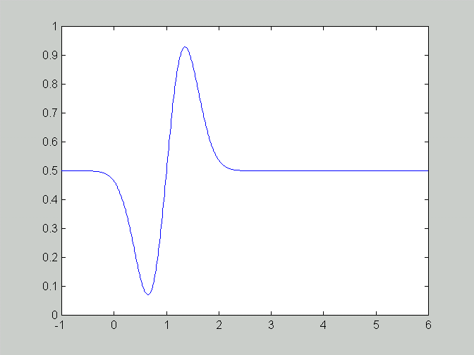
b. To find the maximum of |c(f6(x))|, we need to calculate zeros of the derivative of f6(x):
f6'(x) = [2 - 16(x-1)^2] exp(-4(x-1)^2)The zeros are 1 +/- 1/sqrt(8) and the maximum is reached at x = 1 + 1/sqrt(8) and c_max approx 0.93. The CFL condition is satisfied by choosing Delta t = Delta x.
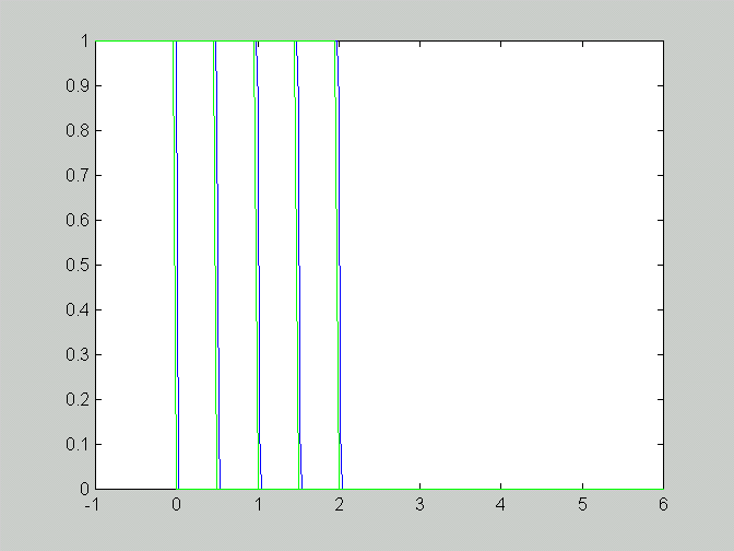
c. Numerical results at t=1,2,3,4 are shown in this figure:
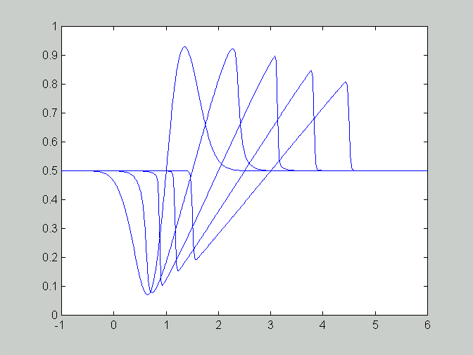
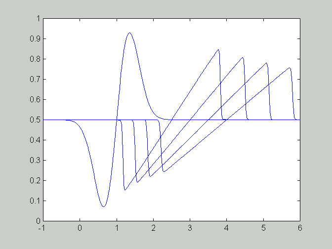
and at the t=6 (rightmost curve below) the solution contains
two discontinuities joined with a line segment:
a. The exact weak solution is the shock:
u(x,t) = 1, if x < t/2 and
u(x,t) = 0, if x > t/2
b. Numerical solution is obtained with the formula:
u(j,n+1) = u(j,n) - [F(u(j,n)) - F(u(j-1,n))] / rho
         = u(j,n) - u(j,n)^2 / 2 + u(j-1,n)^2 / 2
Results of hand calculation:
                    u
n | j=-1 j=0  j=1      j=2  j=3    j=4
---------------------------------------
0 | 1    1    0	       0    0      0      (Initial values)
1 | 1	 1    1/2      0    0      0
2 | 1	 1    7/8      1/8  0      0
3 | 1	 1    127/128  1/2  1/128  0
c. Results from MATLAB agree nicely (array is transposed in comparison to previous array):
   -1.0000    1.0000    1.0000    1.0000    1.0000    1.0000
         0    1.0000    1.0000    1.0000    1.0000    1.0000
    1.0000         0    0.5000    0.8750    0.9922    1.0000
    2.0000         0         0    0.1250    0.5000    0.8672
    3.0000         0         0         0    0.0078    0.1328
    4.0000         0         0         0         0    0.0000
    5.0000         0         0         0         0         0
    6.0000         0         0         0         0         0
More results a little bit later in time (t = 3,4,5,6):
  Columns 1 through 4

  -1.00000000000000   1.00000000000000   1.00000000000000   1.00000000000000
                  0   1.00000000000000   1.00000000000000   1.00000000000000
   1.00000000000000                  0   0.99218750000000   0.99996948242188
   2.00000000000000                  0   0.50000000000000   0.86721801757812
   3.00000000000000                  0   0.00781250000000   0.13278198242188
   4.00000000000000                  0                  0   0.00003051757812
   5.00000000000000                  0                  0                  0
   6.00000000000000                  0                  0                  0

  Columns 5 through 6

   1.00000000000000   1.00000000000000
   1.00000000000000   1.00000000000000
   0.99999999953434   1.00000000000000
   0.99115395545959   0.99996087328233
   0.50000000000000   0.86619308171160
   0.00884604454041   0.13380691828840
   0.00000000046566   0.00003912671767
                  0   0.00000000000000
Transition region grows larger (one Delta x at every new time step),
because the numerical solution computes a kind of average from two previous
points.