28.1.1999
Mikko Kokkonen

Harj. 1, ratkaisut (solutions)

Problem 1

Function coeffmat assembles the left hand size coefficient matrix A of the unknown solution.

>> coeffmat(4)

ans =

  Columns 1 through 12 

     4    -1     0     0    -1     0     0     0     0     0     0     0
    -1     4    -1     0     0    -1     0     0     0     0     0     0
     0    -1     4    -1     0     0    -1     0     0     0     0     0
     0     0    -1     4     0     0     0    -1     0     0     0     0
    -1     0     0     0     4    -1     0     0    -1     0     0     0
     0    -1     0     0    -1     4    -1     0     0    -1     0     0
     0     0    -1     0     0    -1     4    -1     0     0    -1     0
     0     0     0    -1     0     0    -1     4     0     0     0    -1
     0     0     0     0    -1     0     0     0     4    -1     0     0
     0     0     0     0     0    -1     0     0    -1     4    -1     0
     0     0     0     0     0     0    -1     0     0    -1     4    -1
     0     0     0     0     0     0     0    -1     0     0    -1     4
     0     0     0     0     0     0     0     0    -1     0     0     0
     0     0     0     0     0     0     0     0     0    -1     0     0
     0     0     0     0     0     0     0     0     0     0    -1     0
     0     0     0     0     0     0     0     0     0     0     0    -1

  Columns 13 through 16 

     0     0     0     0
     0     0     0     0
     0     0     0     0
     0     0     0     0
     0     0     0     0
     0     0     0     0
     0     0     0     0
     0     0     0     0
    -1     0     0     0
     0    -1     0     0
     0     0    -1     0
     0     0     0    -1
     4    -1     0     0
    -1     4    -1     0
     0    -1     4    -1
     0     0    -1     4

Problem 2

Function rshmat assembles the constant vector (the right hand side of the linear equation group). Matlab-session to find the solution (commands are also in a file):

>> A = coeffmat(4);
>> b = rhsmat([0,0,0,0], [20,40,60,80], [50,20,10,0], [20,40,60,80])

b =

    20
     0
     0
    20
    40
     0
     0
    40
    60
     0
     0
    60
   130
    20
    10
    80

>> s = A \ b;
>> s = reshape(s, 4, 4)';
>> S = [(s(1,1) + 20 + 0)/3 0 0 0 0 (s(1,4) + 20 + 0)/3; ...
     [20; 40; 60; 80] s [20; 40; 60; 80]; ...
     (s(4,1) + 80 + 50)/3 50 20 10 0 (s(4,4) + 80 + 0)/3]

S =

   12.1798         0         0         0         0   12.0374
   20.0000   16.5394   14.2682   14.0273   16.1121   20.0000
   40.0000   31.8894   26.5061   25.7288   30.4212   40.0000
   60.0000   44.5121   34.1379   31.9606   39.8439   60.0000
   80.0000   52.0212   33.5727   28.1318   36.9939   80.0000
   60.6737   50.0000   20.0000   10.0000         0   38.9980

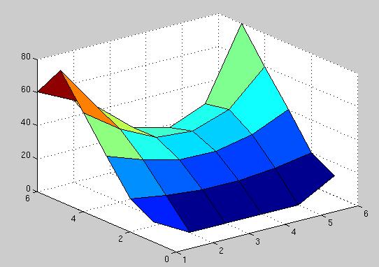
>> surf(S)
>> for j=1:10; view(-20, 10*j); pause; end
>> diary off

Here is the surface plot of the solution:

Problem 3

Function lapsolve contains all the required commands to solve discretized Laplace equation. Matlab-session to solve the problem with interpolated boundary values (commands are also in a file):

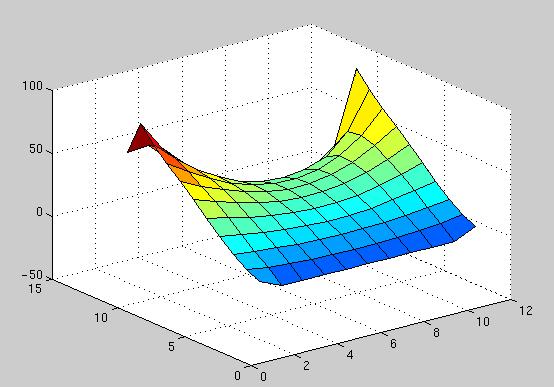
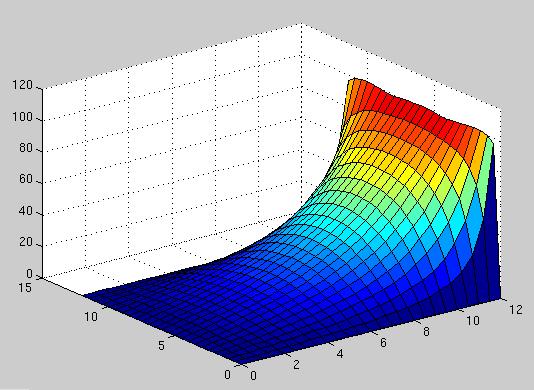
>> pdeg = 4;
>> pbot = polyfit([1 2 3 4], [0 0 0 0], pdeg);
>> pright = polyfit([1 2 3 4], [20 40 60 80], pdeg);
>> ptop = polyfit([1 2 3 4], [50 20 10 0], pdeg);
>> pleft = polyfit([1 2 3 4], [20 40 60 80], pdeg);

>> ix = 0.5:0.5:4.5;
>> itp_bot = polyval(pbot, ix);
>> itp_right = polyval(pright, ix);
>> itp_top = polyval(ptop, ix);
>> itp_left = polyval(pleft, ix);

>> s = lapsolve1(itp_bot, itp_right, itp_top, itp_left);

>> surf(s)

The solution obtained with interpolated boundary values is shown below:

Problem 4

Maple worksheet in HTML for the solution of the heat equation. The output from a Matlab-script which draws a surface plot of the solution is shown below:

Problem 5

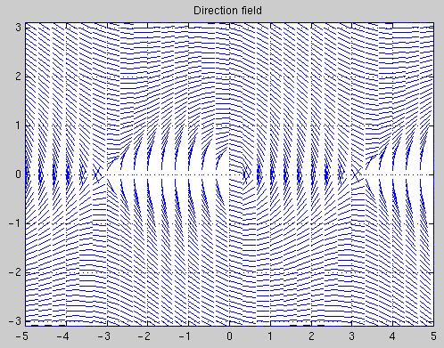
Formulation as a 2-by-2 first-order differential equation system:

y = [ y_1 y_2 ]^T = [ theta theta' ]^T

y' = [ y_1' y_2' ]^T =  [ y_2  -c y_2 - k sin y_1 ]^T

Critical points are the solutions of the equation y' = 0

This implies that y_2 = 0 and -c y_2 - k sin y_1 = 0 <=> sin y_1 = 0 <=> y_1 = n pi

Critical point (0,0): sin y_1 is linearized using the Taylor series:

sin x = x - x^3/3! + ... approx x

Linearized equation

y' = [ y_2  -c y_2 - k y_1 ]^T 

     [  0  1 ] [ y_1 ]
   = [       ] [     ]
     [ -k -c ] [ y_2 ]

Eigenvalues of A are obtained from the equation det(A - m I) = 0 which yields

  -m (-c - m) + k = 0   <=>
  m^2 + c m + k = 0     <=>
  m_1,2 = (-c +/- sqrt( c^2 - 4k )) / 2

Eigenvectors x satistfy the equation Ax = mx <=> (A - mI) x = 0. The equations in the system are dependent and one of the components can be freely chosen. If x_1 is chosen to be 1, then the first equation gives x_2 = m. The eiqenvectors are [1 m_1]^T and [1 m_2]^T.

The classification of a critical point requires the computation of the following quantities:

  p = a_11 + a_22 = -c ( <= 0 )
  q = det A = k ( >= 0 )
  Delta = p^2 - 4k = c^2 - 4k

(0,0) is stable (p <= 0) and attractive if c<0. The type is

node, if c^2 >= 4k
center, if c = 0
spiral point, if c^2 < 4k.

Critical point (pi, 0): The change of variables is required to bring (pi, 0) to origin:

z_1 = y_1 - pi     z_2 = y_2

The diff. equation system is transformed to the form:

z' = y' = [ y_2  -c y_2 - k sin y_1 ]^T = [z_2  -c z_2 - k sin (z_1 + pi)]^T
   = [z_2  -c z_2 + k sin z_1 ]^T

Linearizing the sin z_1 term gives:

y' = [ y_2  -c y_2 + k y_1 ]^T 

     [ 0  1 ] [ y_1 ]
   = [      ] [     ]
     [ k -c ] [ y_2 ]

Eigenvalues are now m_1,2 = (-c +/- sqrt( c^2 + 4k )) / 2 and eigenvectors are [1 m_1]^T and [1 m_2]^T.

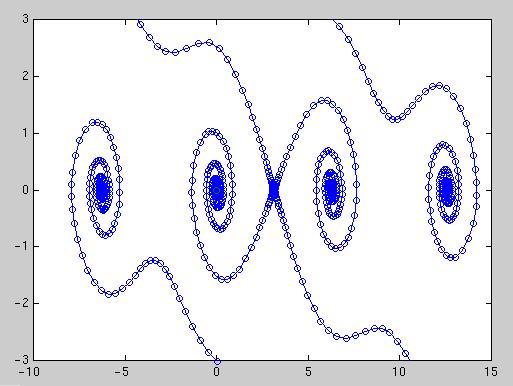
Type of (pi, 0) is always saddle, because roots are always real and of opposite sign and (pi, 0) is unstable, because q = det A = -k < 0.

The rest of the critical points are classified as (0,0) or (pi,0) because of periodicity of sin x.

Ex 1.5c: Phase plane plots

Below is a matlab-script that plots phase-plane for c=0.5 and c=0.25 (both with k=1). First we define the equation system as a matlab-function pendu and the actual script that draws the phase plane plots (two figures separated by a key press) is in the file ex1_5.m.

Phaseplane with c=0.25 and k=1

Phaseplane with c=0.5 and k=1

Ex 1.5d: Direction field plots

The derivative for the direction field plot is obtained by dividing dy_2 / dt by dy_1 / dt. The result is -c -k sin x / y. The actual matlab code for drawing is here.

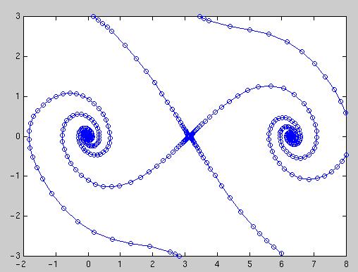
The output from the script is shown below: